Abstract

Apnea of prematurity is a common condition in premature infants that can lead to intermittent hypoxia (IH) episodes, potentially affecting brain development. This study investigated how IH affects cerebellar vascular development using a murine model. We collected and analyzed two complementary datasets: RT-qPCR data measuring expression of angiogenesis-related genes, and 3D immunohistochemistry data quantifying morphological features of the cerebellar vascular network obtained through tissue clearing protocols.

The data was analyzed using generalized linear mixed-effects models. PCR data was modeled using Gaussian distributions, while vascular morphology data used Gamma distributions for continuous measures and negative binomial distributions for count data. All models included random effects to account for pseudo-replication and inter-animal variability.

The repository provides open data, reproducible R code, and key figures used in the associated article. All analyses were conducted in a version-controlled environment using R & {renv}, ensuring full reproducibility of results.

Code

Graphical abstract recapitulating the main findings of this project

My role in this project

1) Managed the data processing, modeling, and hypothesis testing (R/Markdown).

2) Helped write the methodology/statistics part of the paper (in press).

3) Open-sourced the resulting reproducible R code on GitHub and registered it on Zenodo.

Summary

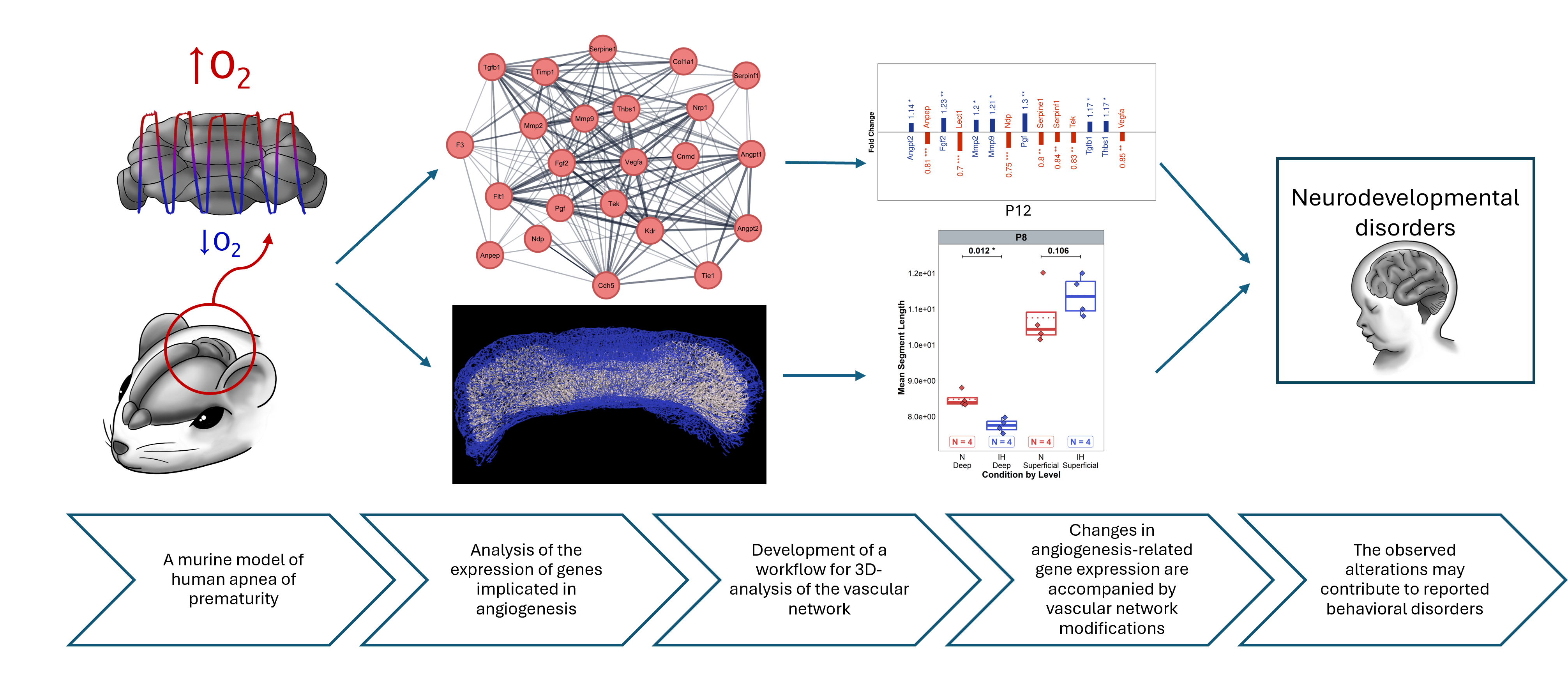
This study used a murine model to investigate how Intermittent Hypoxia (IH), which mimics apnea of prematurity, affects cerebellar vascular development, combining transcriptomic analysis of angiogenesis-related genes with innovative 3D morphological analysis of the cerebellar vascular network. Data was collected across multiple developmental stages (P4, P8, P12, P21, P70), with multiple mice per stage and condition (Normoxia vs IH).

Data

The project analyzed two complementary datasets from a murine model of intermittent hypoxia (IH):

RT-qPCR targeted an angiogenesis-focused gene panel curated via network and pathway analysis using Cytoscape with STRING-DB and ClueGO to prioritize regulators of vascular development. Primers were designed in Primer Express from NCBI sequences, validated by linear regression on serial dilutions, and checked for specificity by NCBI BLAST. Expression was quantified as $\Delta Cq$ .

3D morphological data was obtained from immunohistochemically-stained cerebellar vasculature using innovative tissue clearing protocols. The clearing technique enabled quantification of multiple vascular parameters including total volume, network length, surface area, segment characteristics, and branching patterns, analyzed at both total cerebellar level and stratified by depth (superficial vs deep layers).

Supplementary data

Data preprocessing involved standardizing variable names and metadata using a data dictionary to ensure consistency:

The ‘gene data’ file provides detailed information about the genes analyzed in this study, organized by biological pathways (and how they affect those pathways), and including gene functions, NCBI references, and supporting literature.

Models

Models were fitted using the glmmTMB package (Brooks et al., 2017), and model fit was assessed using a combination of diagnostic plots, statistical tests, and posterior predictive checks using simulated residuals. Model validation employed the DHARMa (Hartig, 2022) and performance (Lüdecke et al., 2021) packages.

Gene expression data ( $\Delta Cq$ values) were modeled using simple linear models per gene (Gaussian likelihood with identity link function), with the condition (IH vs control) as the single fixed effect.

Model equation

$\begin{aligned} \Delta Cq &\sim N \left(\alpha + \beta_{1} Condition, \sigma^2 \right) \end{aligned}$

Equivalent R model

glmmTMB(dcq ~ condition, family = gaussian("identity"))

Model fit

Random sample of 10 models checked for quality of fit using performance::check_model():

Vascular morphology responses were modeled using generalized linear mixed-effects models (GLMMs), with condition, stage, and level (superficial vs deep) as fixed effects. Gamma likelihoods were used for continuous measures, and negative binomial for count data, both with log link functions. Each animal contributed multiple measurements, requiring random-effects to account for pseudo-replication. Cerebellar volume was used as an offset to account for differences in overall brain size between animals and developmental stages. Variance was assumed to vary by developmental stage, and was modeled using a dispersion parameter.

Here is a sample of two of the models we fitted to study changes in cerebellar vascular morphology:

‘Vascular Volume’
‘Branchpoints’

Vascular volume data was modeled using a Gamma distribution to account for strict positivity and positive skewness.

Model equation

$\begin{aligned} Y_{ij} &\sim \mathrm{Gamma}\bigl(\mu_{ij},\phi_{ij}\bigr),\quad \mathrm{Var}(Y_{ij}) = \phi_{ij}\,\mu_{ij}^2,\\ \log(\mu_{ij}) &= \beta_0\\ &\quad + \beta_{\mathrm{condition}}\bigl(\text{condition}_{ij}\bigr)\\ &\quad + \beta_{\mathrm{stage}}\bigl(\text{stage}_{ij}\bigr)\\ &\quad + \beta_{\mathrm{level}}\bigl(\text{level}_{ij}\bigr)\\ &\quad + \beta_{\mathrm{condition}\times\mathrm{stage}} \bigl(\text{condition}_{ij},\text{stage}_{ij}\bigr)\\ &\quad + \beta_{\mathrm{condition}\times\mathrm{level}} \bigl(\text{condition}_{ij},\text{level}_{ij}\bigr)\\ &\quad + \beta_{\mathrm{stage}\times\mathrm{level}} \bigl(\text{stage}_{ij},\text{level}_{ij}\bigr)\\ &\quad + \beta_{\mathrm{condition}\times\mathrm{stage}\times\mathrm{level}} \bigl(\text{condition}_{ij},\text{stage}_{ij},\text{level}_{ij}\bigr)\\ &\quad + \log\!\bigl(\text{cerebellar\_volume}_{ij}\bigr) + b_{\mathrm{mouse}[j]},\\ b_{\mathrm{mouse}[j]} &\sim \mathcal{N}\bigl(0,\sigma^2_{\mathrm{mouse}}\bigr),\\ \log(\phi_{ij}) &= \alpha_0 + \alpha_{\mathrm{stage}}\bigl(\text{stage}_{ij}\bigr). \end{aligned}$

Equivalent R model

mod_vol <- glmmTMB(
  volume ~ condition * stage * level + offset(log(cerebellar_volume)) + (1 | mouse),
  dispformula = ~ stage,
  family = Gamma("log"),
  data = ihc_data |> filter(level != "Total"),
  REML = TRUE
)

Model fit

The number of vascular branchpoints was modeled using a negative binomial distribution to handle overdispersion in count data. The model structure paralleled the volume model, with cerebellar volume as an offset.

Model equation

$\begin{aligned} Y_{ij} &\sim \mathrm{NegBin}_1\bigl(\mu_{ij},\phi_{ij}\bigr),\quad \mathrm{Var}(Y_{ij}) = \mu_{ij}\bigl(1+\phi_{ij}\bigr),\\ \log(\mu_{ij}) &= \beta_0\\ &\quad + \beta_{\mathrm{condition}}\bigl(\text{condition}_{ij}\bigr)\\ &\quad + \beta_{\mathrm{stage}}\bigl(\text{stage}_{ij}\bigr)\\ &\quad + \beta_{\mathrm{level}}\bigl(\text{level}_{ij}\bigr)\\ &\quad + \beta_{\mathrm{condition}\times\mathrm{stage}} \bigl(\text{condition}_{ij},\text{stage}_{ij}\bigr)\\ &\quad + \beta_{\mathrm{condition}\times\mathrm{level}} \bigl(\text{condition}_{ij},\text{level}_{ij}\bigr)\\ &\quad + \beta_{\mathrm{stage}\times\mathrm{level}} \bigl(\text{stage}_{ij},\text{level}_{ij}\bigr)\\ &\quad + \beta_{\mathrm{condition}\times\mathrm{stage}\times\mathrm{level}} \bigl(\text{condition}_{ij},\text{stage}_{ij},\text{level}_{ij}\bigr)\\ &\quad + \log\!\bigl(\text{cerebellar\_volume}_{ij}\bigr) + b_{\mathrm{mouse}[j]},\\ b_{\mathrm{mouse}[j]} &\sim \mathcal{N}\bigl(0,\sigma^2_{\mathrm{mouse}}\bigr),\\ \log(\phi_{ij}) &= \alpha_0 + \alpha_{\mathrm{stage}}\bigl(\text{stage}_{ij}\bigr). \end{aligned}$

Equivalent R model

mod_branchpoints <- glmmTMB(
  branchpoints ~ condition * stage * level + offset(log(cerebellar_volume)) + (1 | mouse),
  dispformula = ~ stage,
  family = nbinom1("log"),
  data = ihc_data |> filter(level != "Total"),
  REML = TRUE
)

Model fit

Hypotheses

The central research question investigated whether intermittent hypoxia (IH) exposure, mimicking apnea of prematurity, affects cerebellar vascular development through both transcriptomic changes in angiogenesis-related genes and morphological alterations in the cerebellar vascular network.

Contrasts for hypotheses of interest were tested with emmeans (Lenth, 2022).

We hypothesized that intermittent hypoxia would alter expression of genes involved in angiogenesis pathways, potentially showing both pro- and anti-angiogenic responses depending on the specific gene and developmental stage.

The analysis focused on identifying genes that showed significant differential expression between IH and control conditions across developmental stages. Fold changes were calculated and significance was assessed using the fitted linear models, with genes classified as upregulated, downregulated, or unchanged based on p-values and effect sizes.

Here’s a general overview of the gene expression changes between IH and control, across developmental stages:

Timeline of gene expression changes across developmental stages, providing insights into the temporal dynamics of the transcriptomic response to intermittent hypoxia:

Timeline of the gene’s putative effects (anti- vs pro-angiogenic) across developmental stages (based on existing literature):

We hypothesized that intermittent hypoxia would affect the morphological development of the cerebellar vascular network, potentially altering vascular density, complexity, and branching patterns.

Vascular Volume
Branchpoints

Analysis of total vascular volume tested whether IH exposure affected overall vascularization of the cerebellum, accounting for developmental stage differences and normalizing for brain size using cerebellar volume as an offset.

emmeans(mod_vol, specs = "condition", type = "response") |> 
  contrast(method = "pairwise", adjust = "none", infer = TRUE) |> 
  as.data.frame()

data.frame [1 x 9]

contrast	ratio	SE	df	lower.CL	upper.CL	null	t.ratio	p.value
N / IH	0.411	0.179	55	0.172	0.984	1	−2.042	0.046

emmeans(mod_vol, specs = ~ condition | stage, type = "response") |> 
  contrast(method = "pairwise", adjust = "none", infer = TRUE) |> 
  as.data.frame()

data.frame [4 x 10]

contrast	stage	ratio	SE	df	lower.CL	upper.CL	null	t.ratio	p.value
N / IH	P4	0.171	0.133	55	0.036	0.812	1	−2.272	0.027
N / IH	P8	0.457	0.374	55	0.089	2.357	1	−0.956	0.343
N / IH	P12	0.71	0.696	55	0.099	5.069	1	−0.349	0.728
N / IH	P21	0.513	0.459	55	0.085	3.085	1	−0.745	0.459

emmeans(mod_vol, specs = ~ condition | level, by = "stage", type = "response") |> 
  contrast(method = "pairwise", adjust = "none", infer = TRUE) |> 
  as.data.frame()

data.frame [8 x 11]

contrast	level	stage	ratio	SE	df	lower.CL	upper.CL	null	t.ratio	p.value
N / IH	Deep	P4	0.219	0.173	55	0.045	1.066	1	−1.923	0.06
N / IH	Superficial	P4	0.134	0.105	55	0.027	0.649	1	−2.551	0.014
N / IH	Deep	P8	0.725	0.633	55	0.126	4.175	1	−0.368	0.714
N / IH	Superficial	P8	0.288	0.253	55	0.05	1.67	1	−1.419	0.162
N / IH	Deep	P12	1.068	1.233	55	0.105	10.811	1	0.057	0.955
N / IH	Superficial	P12	0.472	0.546	55	0.046	4.794	1	−0.649	0.519
N / IH	Deep	P21	0.373	0.36	55	0.054	2.581	1	−1.021	0.312
N / IH	Superficial	P21	0.706	0.684	55	0.101	4.92	1	−0.359	0.721

The branchpoint analysis examined whether IH affected vascular network complexity and branching architecture, testing for condition effects across developmental stages while controlling for overall brain size.

emmeans(mod_branchpoints, specs = "condition", type = "response") |> 
  contrast(method = "pairwise", adjust = "none", infer = TRUE) |> 
  as.data.frame()

data.frame [1 x 9]

contrast	ratio	SE	df	lower.CL	upper.CL	null	t.ratio	p.value
N / IH	0.744	0.111	55	0.553	1.003	1	−1.987	0.052

emmeans(mod_branchpoints, specs = ~ condition | stage, type = "response") |> 
  contrast(method = "pairwise", adjust = "none", infer = TRUE) |> 
  as.data.frame()

data.frame [4 x 10]

contrast	stage	ratio	SE	df	lower.CL	upper.CL	null	t.ratio	p.value
N / IH	P4	0.599	0.139	55	0.376	0.954	1	−2.208	0.031
N / IH	P8	1.072	0.181	55	0.764	1.504	1	0.412	0.682
N / IH	P12	0.43	0.202	55	0.168	1.102	1	−1.798	0.078
N / IH	P21	1.112	0.249	55	0.71	1.742	1	0.475	0.637

emmeans(mod_branchpoints, specs = ~ condition | level, by = "stage", type = "response") |> 
  contrast(method = "pairwise", adjust = "none", infer = TRUE) |> 
  as.data.frame()

data.frame [8 x 11]

contrast	level	stage	ratio	SE	df	lower.CL	upper.CL	null	t.ratio	p.value
N / IH	Deep	P4	0.626	0.115	55	0.433	0.905	1	−2.548	0.014
N / IH	Superficial	P4	0.572	0.219	55	0.266	1.23	1	−1.461	0.15
N / IH	Deep	P8	1.054	0.161	55	0.776	1.431	1	0.345	0.732
N / IH	Superficial	P8	1.091	0.255	55	0.682	1.743	1	0.371	0.712
N / IH	Deep	P12	0.551	0.304	55	0.182	1.667	1	−1.079	0.285
N / IH	Superficial	P12	0.336	0.242	55	0.079	1.42	1	−1.517	0.135
N / IH	Deep	P21	0.865	0.133	55	0.636	1.177	1	−0.945	0.349
N / IH	Superficial	P21	1.43	0.525	55	0.685	2.984	1	0.974	0.334

References

Brooks, M. E., Kristensen, K., van Benthem, K. J., Magnusson, A., Berg, C. W., Nielsen, A., Skaug, H. J., Maechler, M., & Bolker, B. M. (2017). glmmTMB balances speed and flexibility among packages for zero-inflated generalized linear mixed modeling. The R Journal, 9(2), 378–400. https://journal.r-project.org/archive/2017/RJ-2017-066/index.html

Hartig, F. (2022). DHARMa: Residual diagnostics for hierarchical (multi-level / mixed) regression models. https://CRAN.R-project.org/package=DHARMa

Lenth, R. V. (2022). Emmeans: Estimated marginal means, aka least-squares means. https://CRAN.R-project.org/package=emmeans

Lüdecke, D., Ben-Shachar, M. S., Patil, I., Waggoner, P., & Makowski, D. (2021). performance: An R package for assessment, comparison and testing of statistical models. Journal of Open Source Software, 6(60), 3139. https://doi.org/10.21105/joss.03139