Abstract

Alzheimer’s disease (AD) is associated with mitochondrial dysfunction and hypoxia-like signaling that can induce BNIP3, a key mediator of mitophagy and cell death. This study quantified BNIP3 immunoreactivity in neuronal soma and axonal projections across multiple brain regions (entorhinal cortex, CA3, dentate gyrus) in an established AD rat model compared to matched controls. We analyzed brightfield immunohistochemistry data from 24 rats (12 AD model, 12 controls) across three age groups (3, 12, 18 months), measuring optical density with background correction.

The data was analyzed using generalized linear mixed-effects models with Gamma likelihoods and random effects captured animal-level and section-level variability, while fixed effects tested genotype, age, and brain region effects, and their interactions. Model fit was rigorously assessed using diagnostic plots, statistical tests, and posterior predictive checks.

The repository provides open data, code, and key figures used in the associated article. All figures and tables were generated reproducibly from R Markdown in a version-controlled environment.

Article Code

Graphical abstract recapitulating the main findings of this project

Summary

My role in this project

1) Managed the code for data processing, modeling, and hypothesis testing.

2) Helped write the methodology/statistics part of the paper (Rodriguez-Duboc et al., 2025).

3) Open-sourced the resulting code on GitHub and registered it on Zenodo.

Data

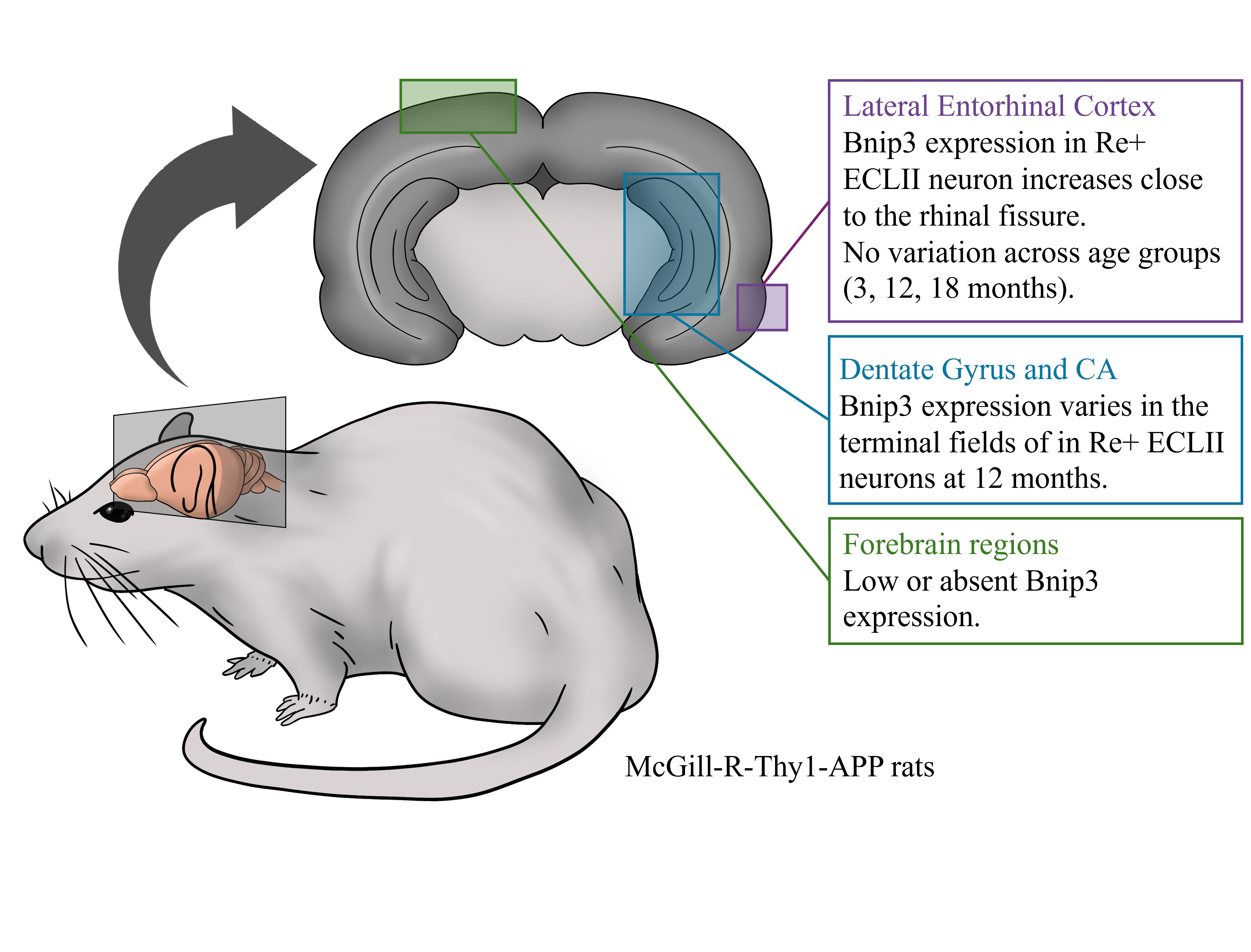
The project analyzed brightfield immunohistochemistry (IHC) data quantified as optical density (OD) measurements from brain tissue sections. Data was collected from 24 rats (12 AD model, 12 controls) across three age groups (3, 12, 18 months) to measure BNIP3 protein expression in neuronal soma and axonal projections. Each animal contributed 7-8 tissue sections covering specific brain regions (entorhinal cortex, CA3, dentate gyrus), with background correction applied by subtracting deep layer measurements from raw OD values. The dataset included hierarchical structure with measurements nested within sections, sections within animals, creating pseudo-replication that required mixed-effects modeling approaches.

Data preprocessing involved standardizing variable names and metadata using a data dictionary to ensure consistent analysis workflows. The final dataset captured both cellular (soma) and projection field (molecular layer) measurements across genotype, age, and brain region factors.

Models

Optical Density (OD) data was modeled using a Gamma distribution to account for the data’s strict positivity and positive skewness, with a log link function.

Generalized Linear Mixed Models (GLMMs) were used to model the data, using random effects to account for pseudo-replication and the hierarchical nature of the data. For all models, categorical predictors were dummy-coded with a reference level: genotype (Wild-Type) and age (3 months). Models were fitted using the glmmTMB package (Brooks et al., 2017).

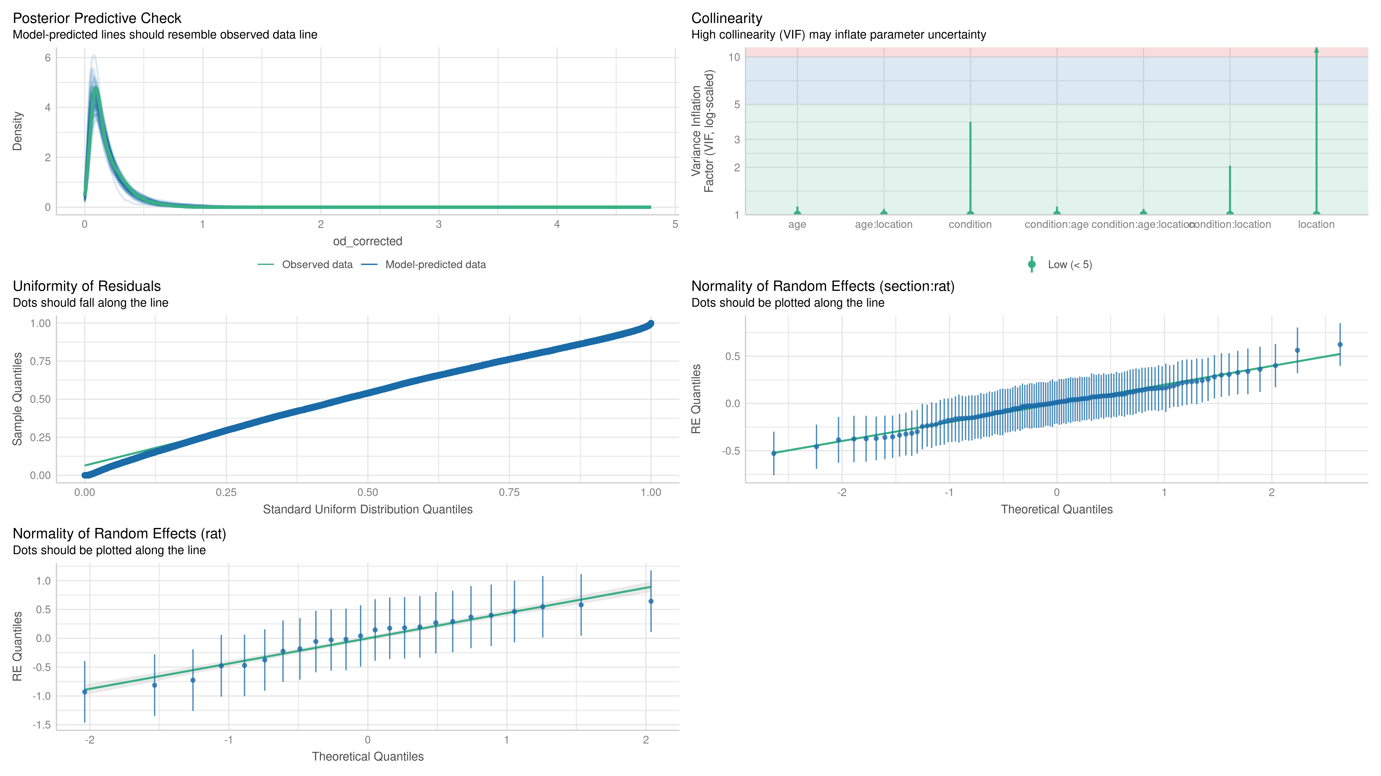
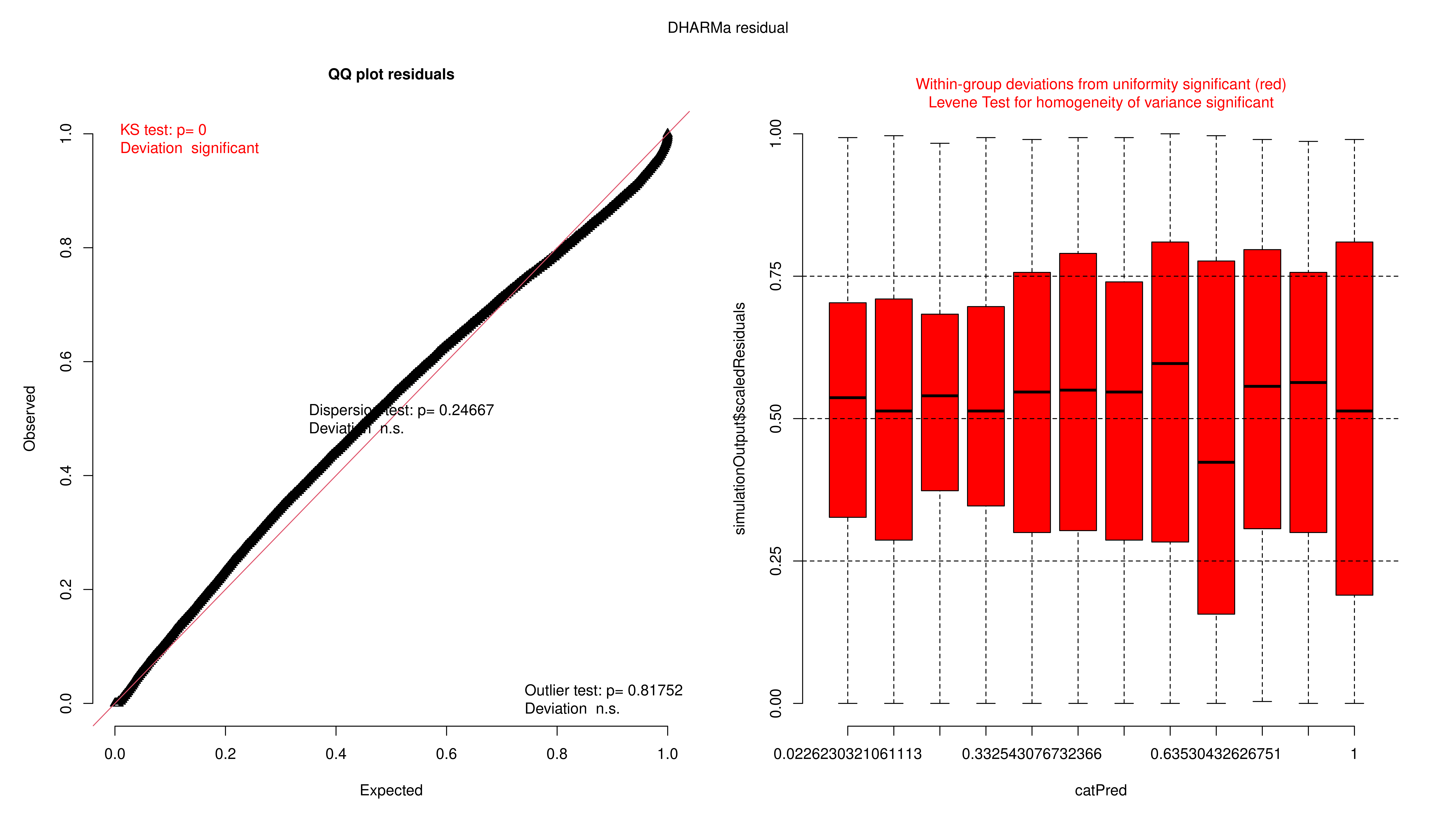
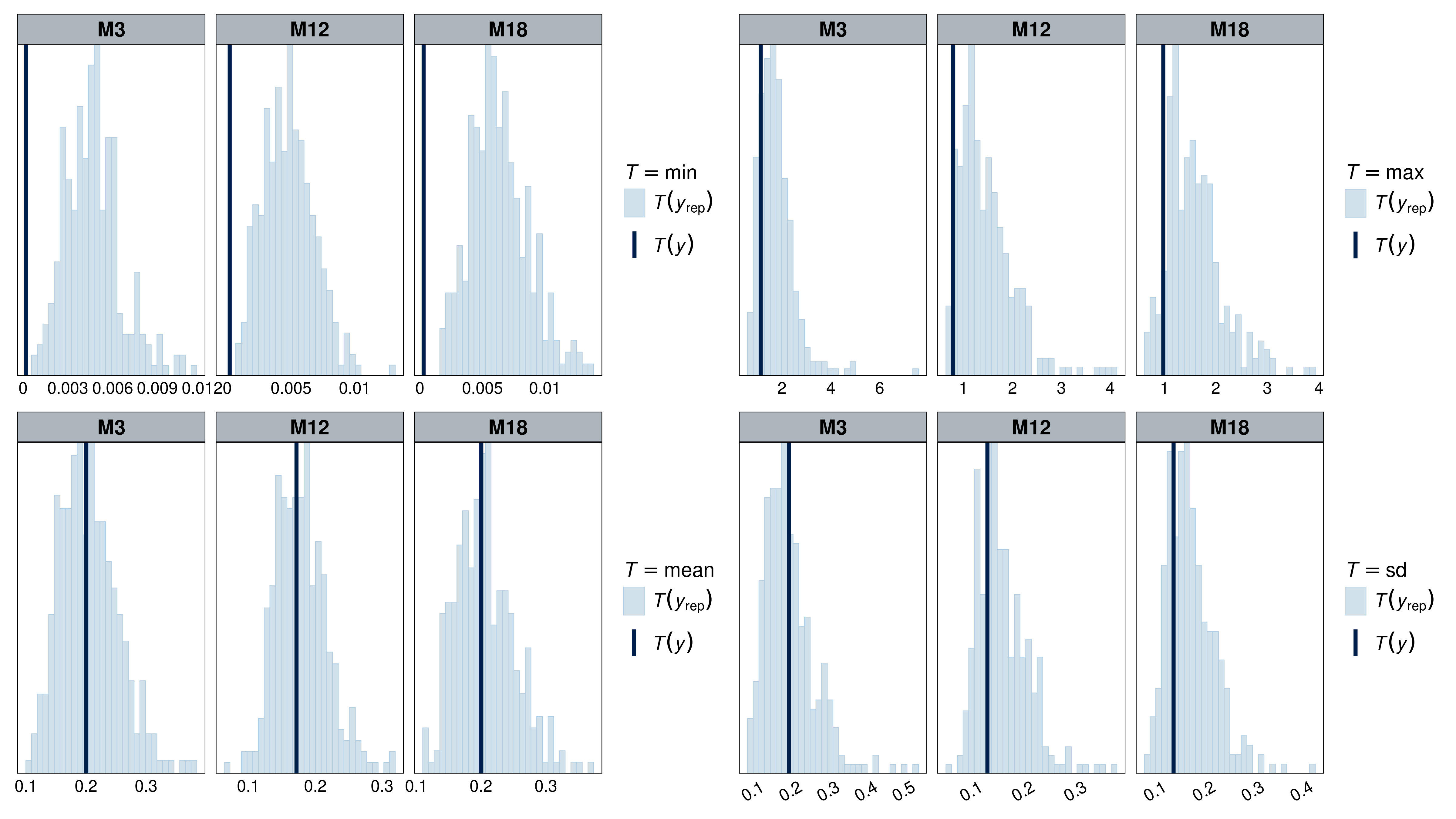
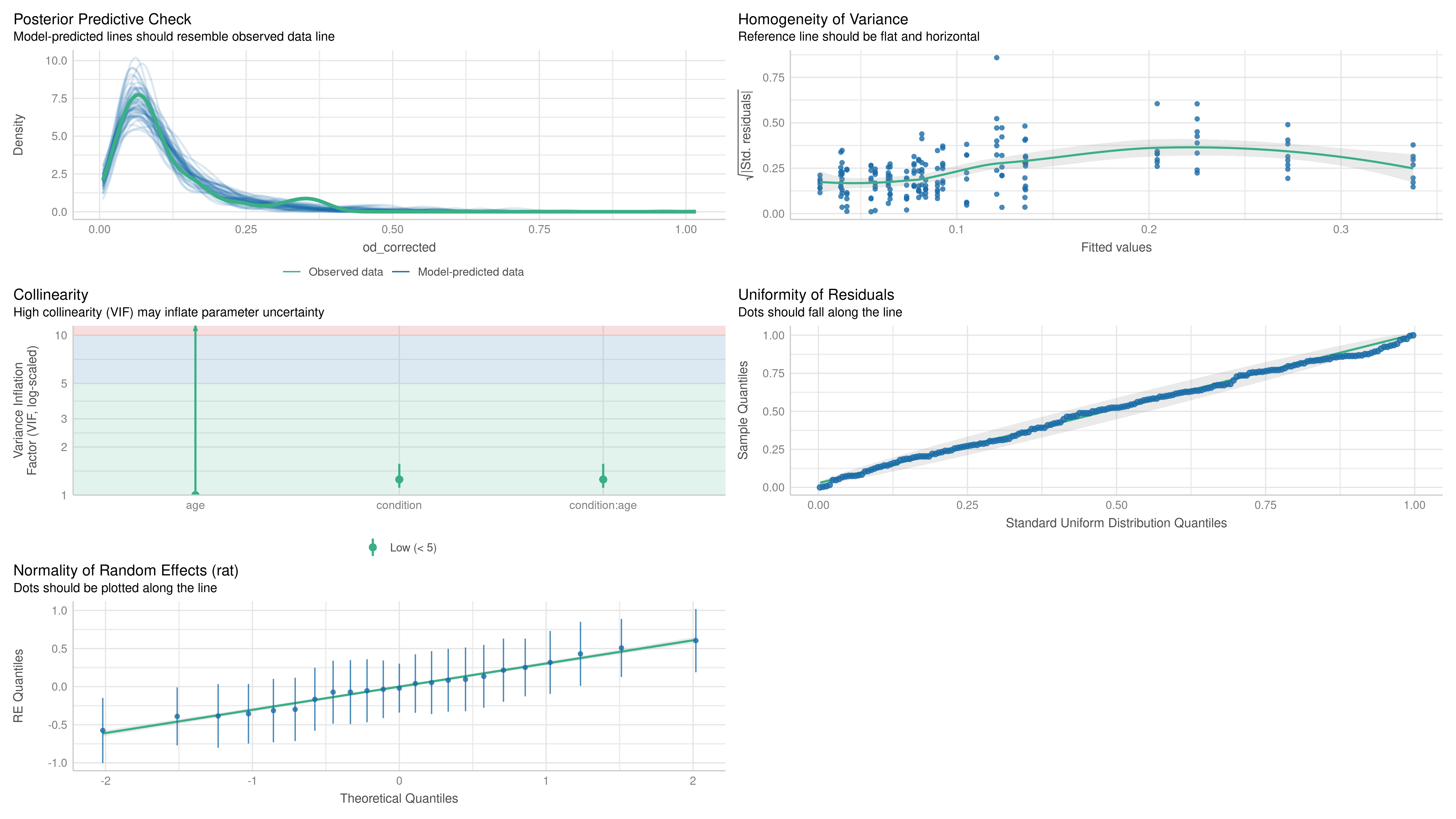
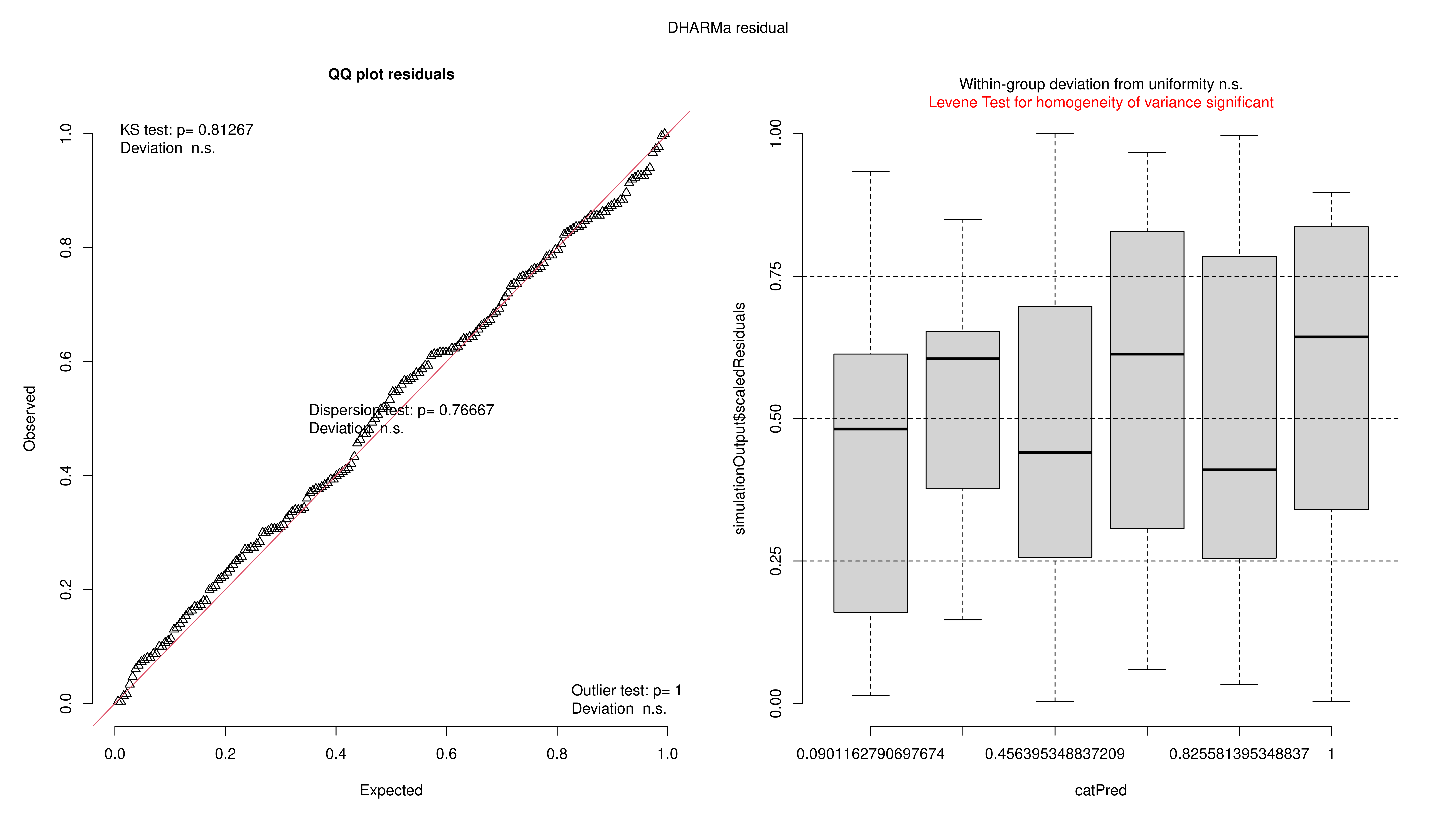
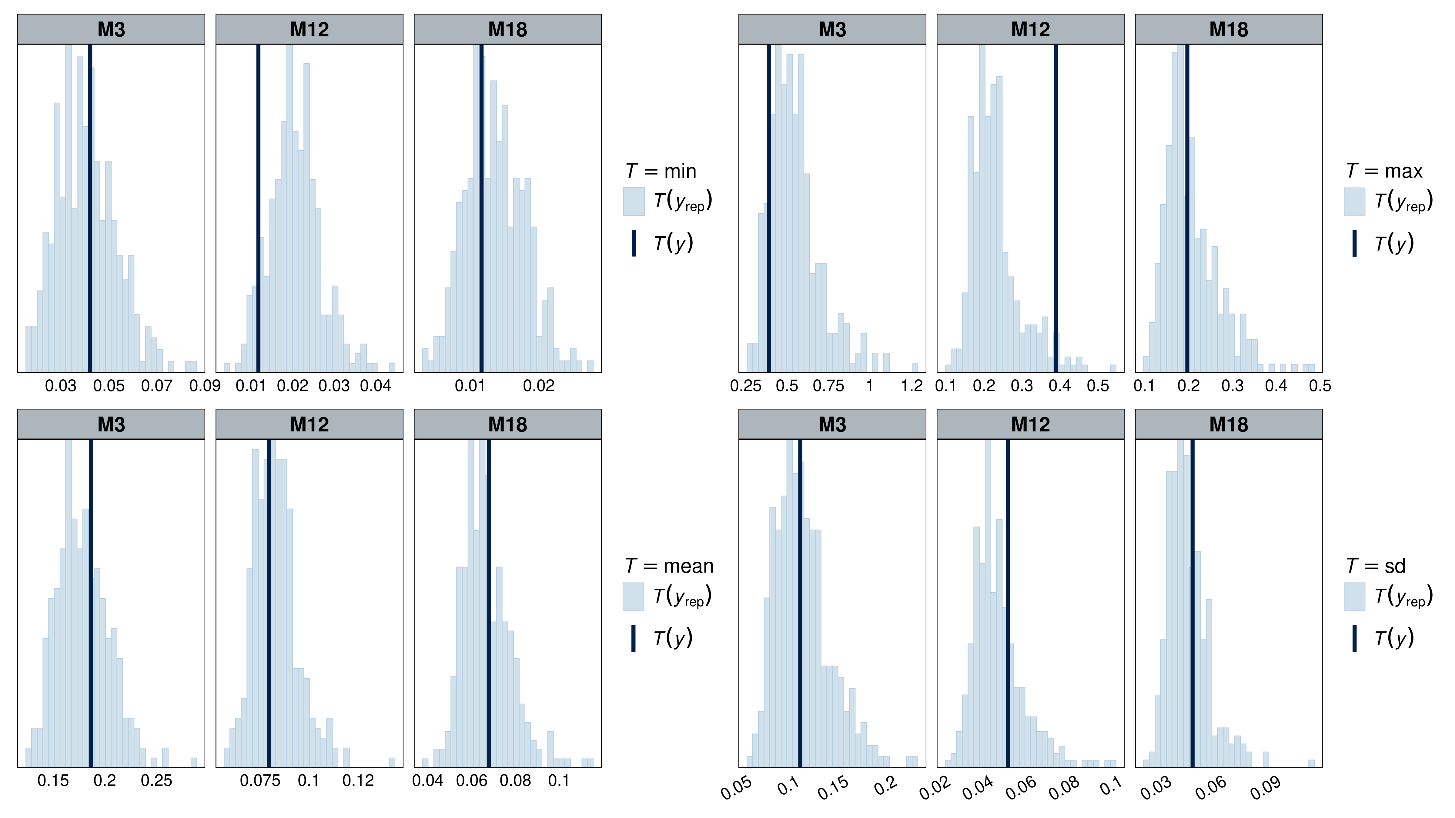
Model fit was assessed using a combination of plots (normality, homoscedasticity, normality of residuals, collinearity), statistical tests (Levenne, KS, dispersion), and posterior predictive checks on simple statistics (min, max, mean, sd) using simulated residuals. Model fit was assessed using the DHARMa (Hartig, 2022) and performance (Lüdecke et al., 2021) packages.

Two models were fitted on the OD data, one for the soma and one for the molecular layer (terminal fields):

‘Soma’ model
‘Molecular Layer’ model

We modeled the OD of individual neuronal somata ( $Y_{ijk}$ ) using genotype, age, and brain area (LEC vs. MEC) as fixed effects, along with all their interactions. Random intercepts were included for each rat (j) and for each tissue section (k) nested within each rat.

Model equation

$\begin{aligned} Y_{ijk} &\sim \mathrm{Gamma}\bigl(\mu_{ijk},\phi\bigr),\quad \mathrm{Var}(Y_{ijk}) = \phi\,\mu_{ijk}^2,\\ \log(\mu_{ijk}) &= \beta_0\\ &\quad + \beta_{\mathrm{Genotype}}\bigl(\text{genotype}_{ijk}\bigr)\\ &\quad + \beta_{\mathrm{Age}}\bigl(\text{age}_{ijk}\bigr)\\ &\quad + \beta_{\mathrm{Area}}\bigl(\text{area}_{ijk}\bigr)\\ &\quad + \beta_{\mathrm{Genotype}\times\mathrm{Age}}\bigl(\text{genotype}_{ijk},\text{age}_{ijk}\bigr)\\ &\quad + \beta_{\mathrm{Genotype}\times\mathrm{Area}}\bigl(\text{genotype}_{ijk},\text{area}_{ijk}\bigr)\\ &\quad + \beta_{\mathrm{Age}\times\mathrm{Area}}\bigl(\text{age}_{ijk},\text{area}_{ijk}\bigr)\\ &\quad + \beta_{\mathrm{Genotype}\times\mathrm{Age}\times\mathrm{Area}}\bigl(\text{genotype}_{ijk},\text{age}_{ijk},\text{area}_{ijk}\bigr)\\ &\quad + b_{\mathrm{rat}[j]} + b_{\mathrm{rat:section}[j,k]},\\ b_{\mathrm{rat}[j]} &\sim \mathcal{N}\bigl(0,\sigma^2_{\mathrm{rat}}\bigr),\quad b_{\mathrm{rat:section}[j,k]} \sim \mathcal{N}\bigl(0,\sigma^2_{\mathrm{rat:section}}\bigr). \end{aligned}$

Equivalent R model

glmmTMB::glmmTMB(
  od_corrected ~ genotype * age * area + (1 | rat / section),
  family = Gamma("log"),
  data = od_data$soma,
  REML = TRUE
)

Model fit

Posterior Predictive Checks on simple stats for the 'Soma' model

To model the OD of the terminal fields ( $Y_{ij}$ ), the fixed effects included genotype, age, and their interaction. A random intercept for each rat (j) was included to account for inter-animal variability.

Model equation

$\begin{aligned} Y_{ij} &\sim \mathrm{Gamma}\bigl(\mu_{ij},\phi\bigr),\quad \mathrm{Var}(Y_{ij}) = \phi\,\mu_{ij}^2,\\ \log(\mu_{ij}) &= \beta_0\\ &\quad + \beta_{\mathrm{Genotype}}\bigl(\text{genotype}_{ij}\bigr)\\ &\quad + \beta_{\mathrm{Age}}\bigl(\text{age}_{ij}\bigr)\\ &\quad + \beta_{\mathrm{Genotype}\times\mathrm{Age}}\bigl(\text{genotype}_{ij},\text{age}_{ij}\bigr)\\ &\quad + b_{\mathrm{rat}[j]},\\ b_{\mathrm{rat}[j]} &\sim \mathcal{N}\bigl(0,\sigma^2_{\mathrm{rat}}\bigr). \end{aligned}$

Equivalent R model

glmmTMB(
    od_corrected ~ genotype * age + (1 | rat),
    family = Gamma("log"),
    data = od_data$ml,
    REML = TRUE
)

Model fit

Performance plots for the 'Molecular Layer' model

DHARMa plots for the 'Molecular Layer' model

Posterior Predictive Checks on simple stats for the 'Molecular Layer' model

Hypotheses

Contrasts for hypotheses of interest were tested with emmeans (Lenth, 2022), with the Holm method to adjust for multiple comparisons.

Soma
Molecular Layer

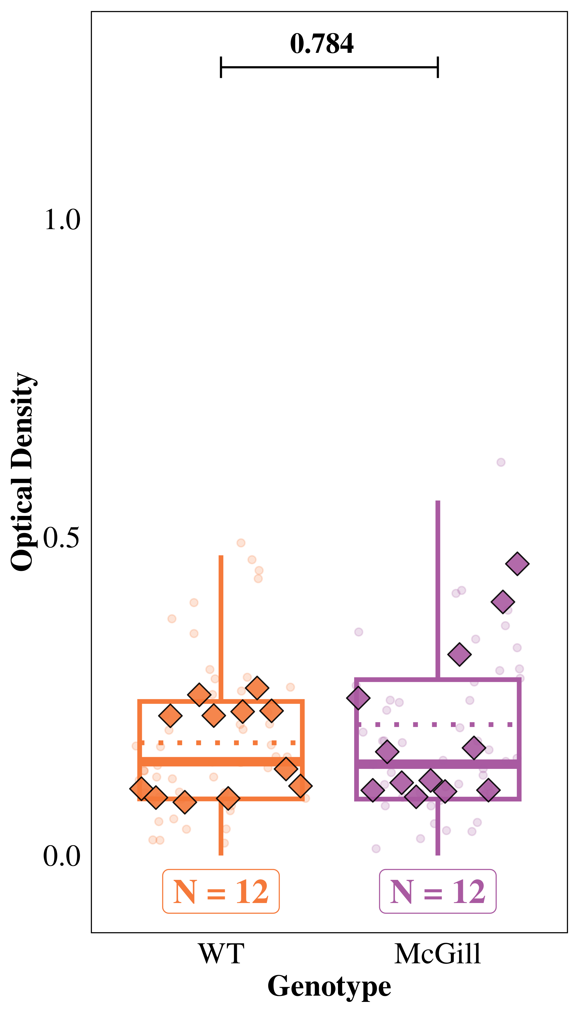
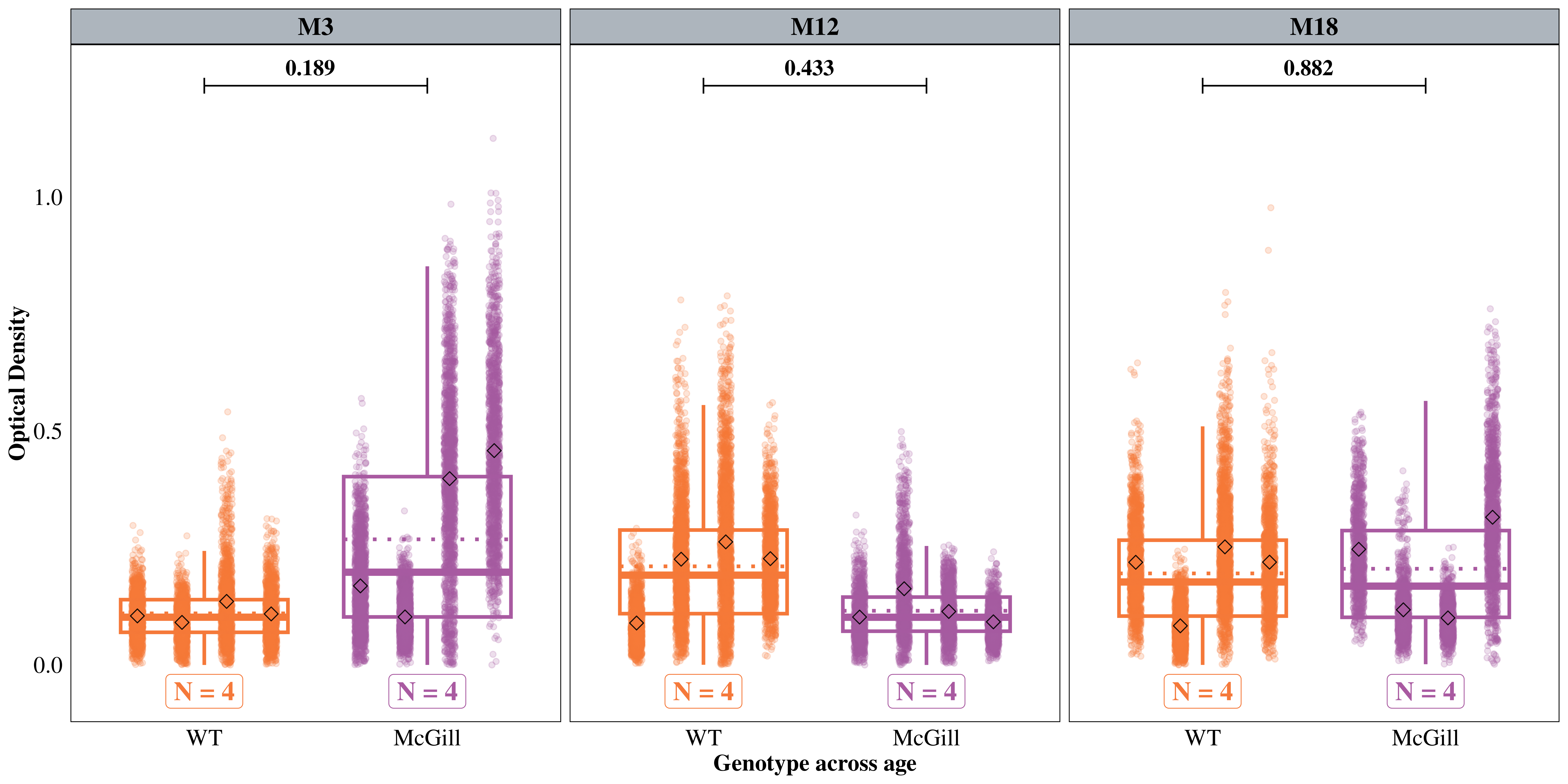
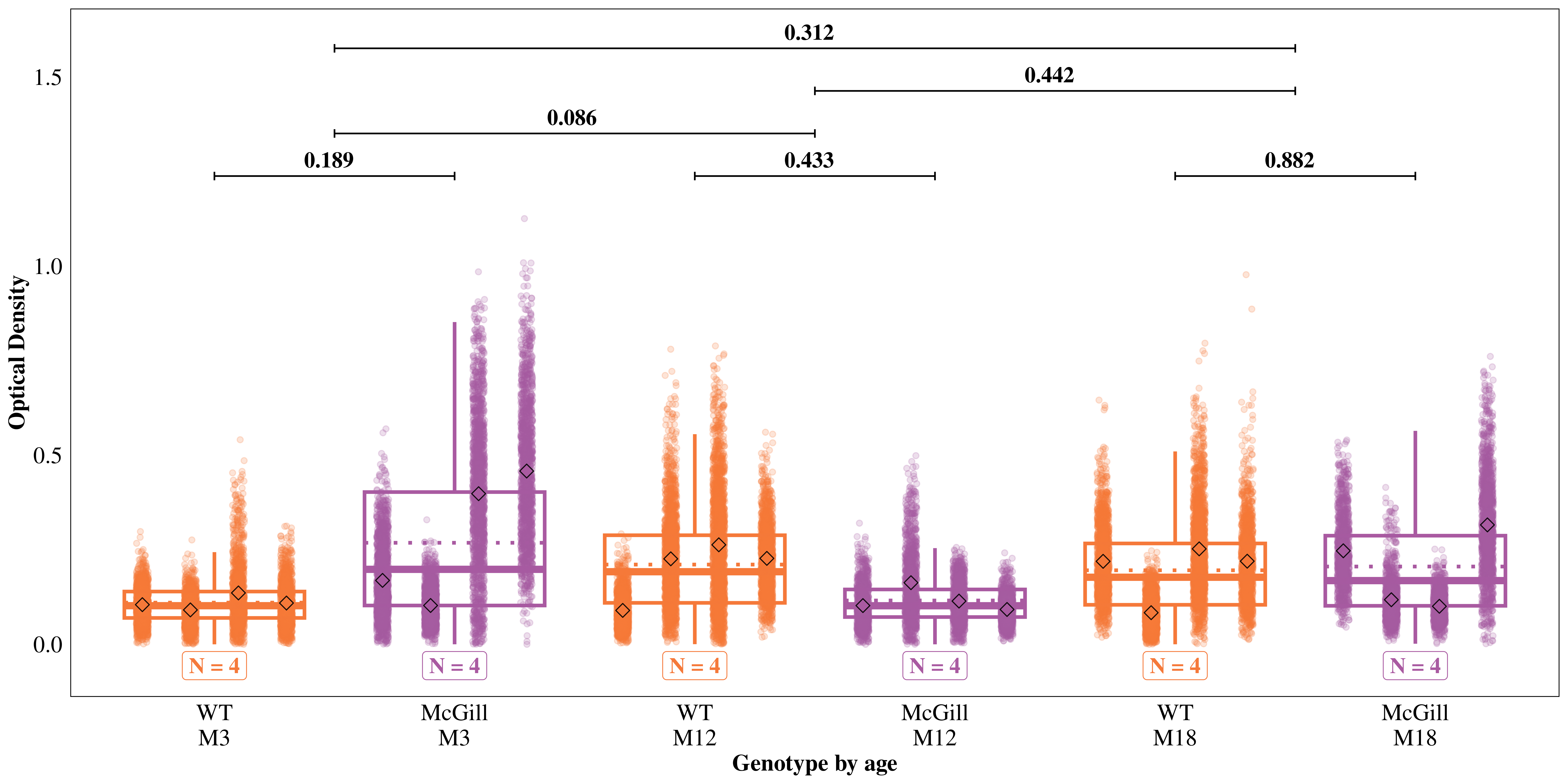
Since Reelin neurons have high metabolism, we hypothesized a higher Bnip3 expression in the soma of LEC/MEC neurons in AD rats, and the difference should be higher in older rats. We used the ‘Soma’ model to test these hypotheses.

emmeans(mod_soma, specs = "genotype", type = "response") |> 
    contrast(method = "pairwise", adjust = "holm", infer = TRUE)

 contrast    ratio    SE  df asymp.LCL asymp.UCL null z.ratio p.value
 WT / McGill 0.943 0.202 Inf     0.619      1.44    1  -0.274  0.7842

Results are averaged over the levels of: age, area 
Confidence level used: 0.95 
Intervals are back-transformed from the log scale 
Tests are performed on the log scale

Annotated boxplots comparing BNIP3 expression in AD and control rats across age groups

emmeans(mod_soma, specs = ~ genotype | age, type = "response") |> 
    contrast(method = "pairwise", adjust = "none", infer = TRUE) |> 
    as.data.frame() |> 
    modify_at("p.value", \(x) p.adjust(x, method = "holm"))

age = M3:
 contrast     ratio     SE  df asymp.LCL asymp.UCL null z.ratio p.value
 WT / McGill 0.5012 0.1862 Inf    0.2420     1.038    1  -1.859  0.1891

age = M12:
 contrast     ratio     SE  df asymp.LCL asymp.UCL null z.ratio p.value
 WT / McGill 1.5831 0.5882 Inf    0.7643     3.279    1   1.236  0.4326

age = M18:
 contrast     ratio     SE  df asymp.LCL asymp.UCL null z.ratio p.value
 WT / McGill 1.0566 0.3927 Inf    0.5100     2.189    1   0.148  0.8822

Results are averaged over the levels of: area 
Confidence level used: 0.95 
Intervals are back-transformed from the log scale 
Tests are performed on the log scale

Annotated boxplots comparing BNIP3 expression in AD and control rats within age groups

emmeans(mod_soma, specs = ~ genotype | age, type = "response") |>
    contrast(interaction = "pairwise", by = NULL, adjust = "none", infer = TRUE) |> 
    as.data.frame() |> 
    modify_at("p.value", \(x) p.adjust(x, method = "holm"))

 genotype_pairwise age_pairwise  ratio     SE  df asymp.LCL asymp.UCL null z.ratio p.value
 WT / McGill        M3 / M12     0.3166 0.1664 Inf    0.1131     0.887    1  -2.189  0.0858
 WT / McGill        M3 / M18     0.4744 0.2493 Inf    0.1694     1.329    1  -1.419  0.3118
 WT / McGill        M12 / M18    1.4983 0.7874 Inf    0.5349     4.197    1   0.769  0.4417

Results are averaged over the levels of: area 
Confidence level used: 0.95 
Intervals are back-transformed from the log scale 
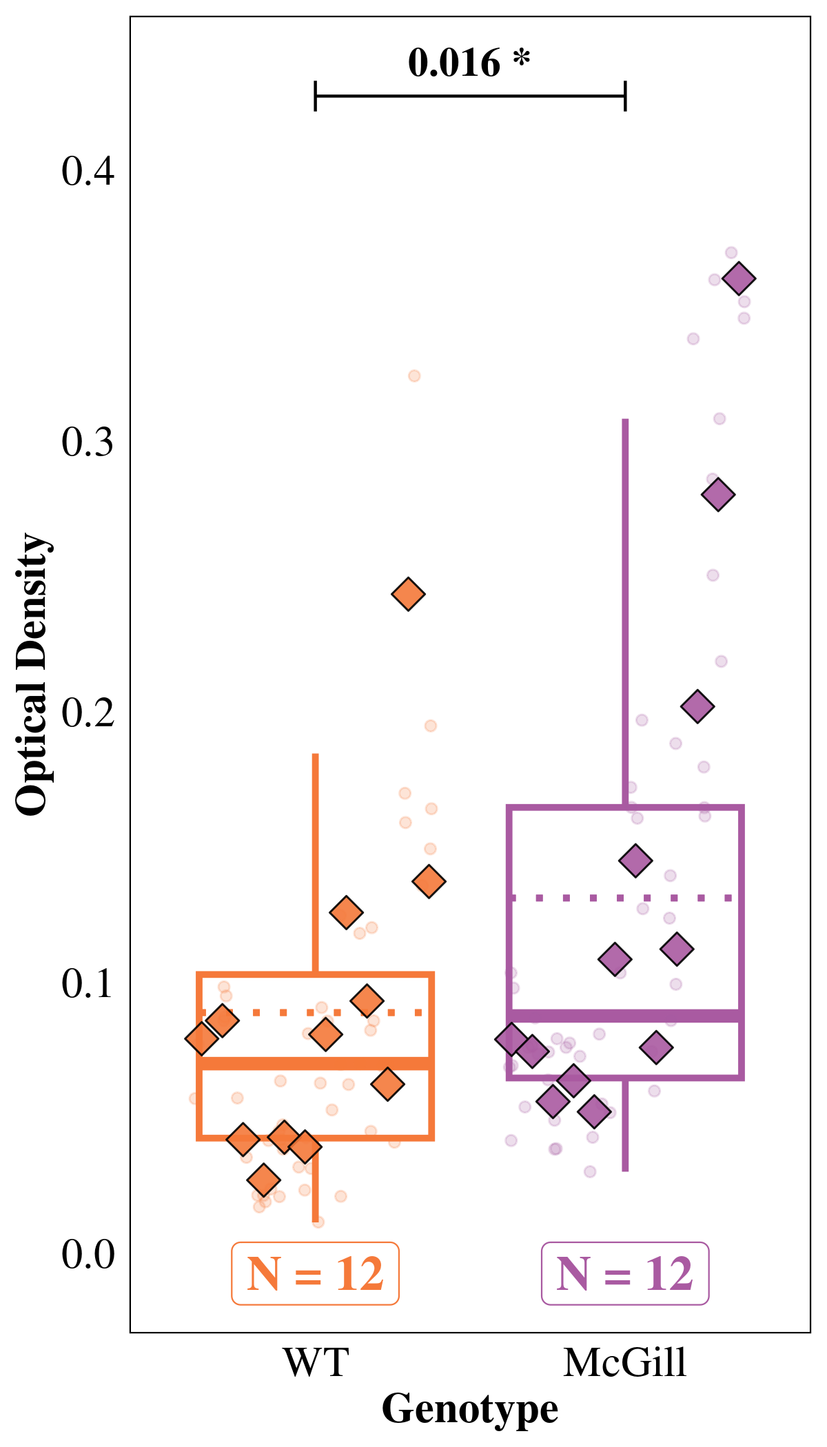
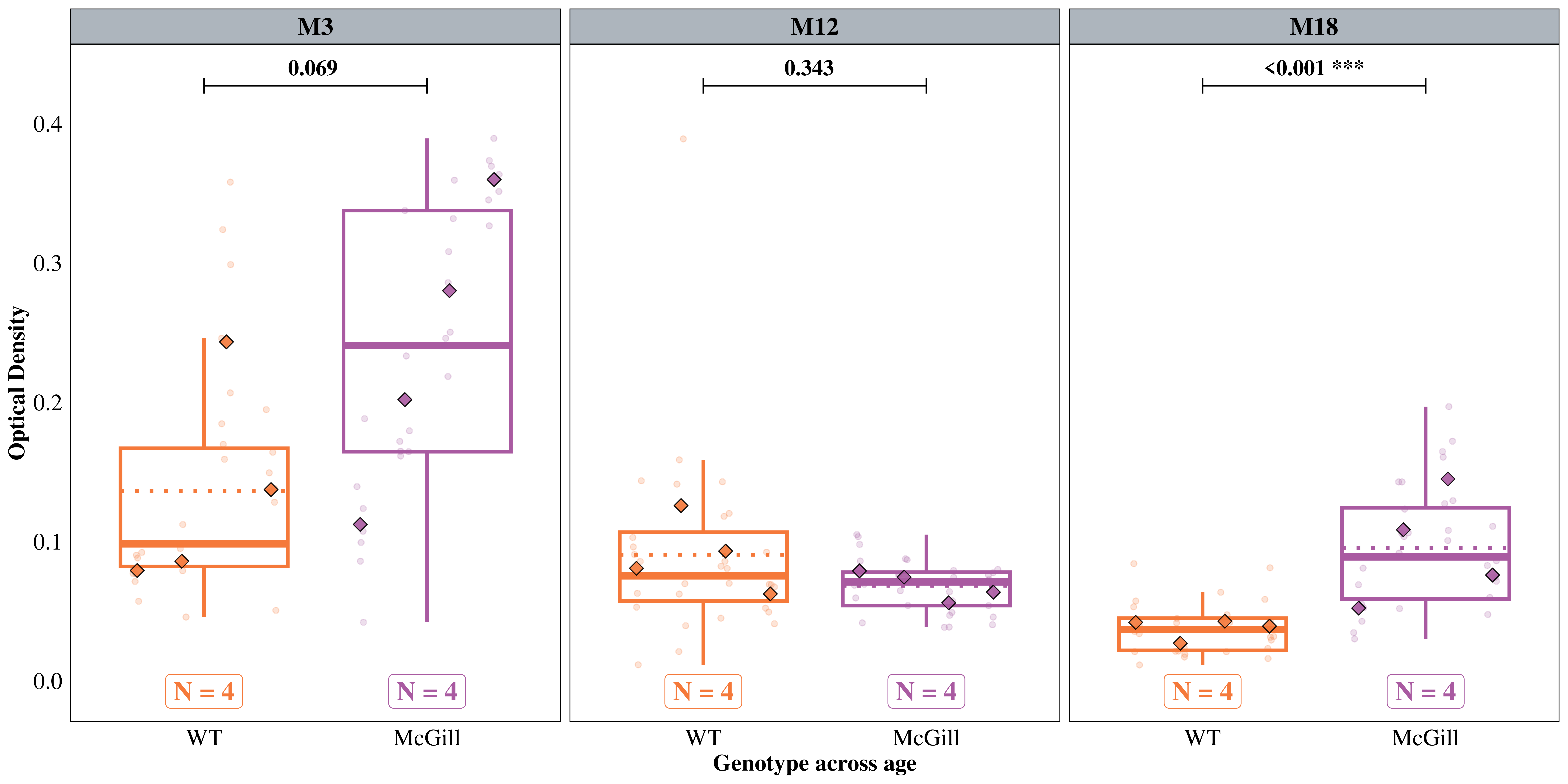
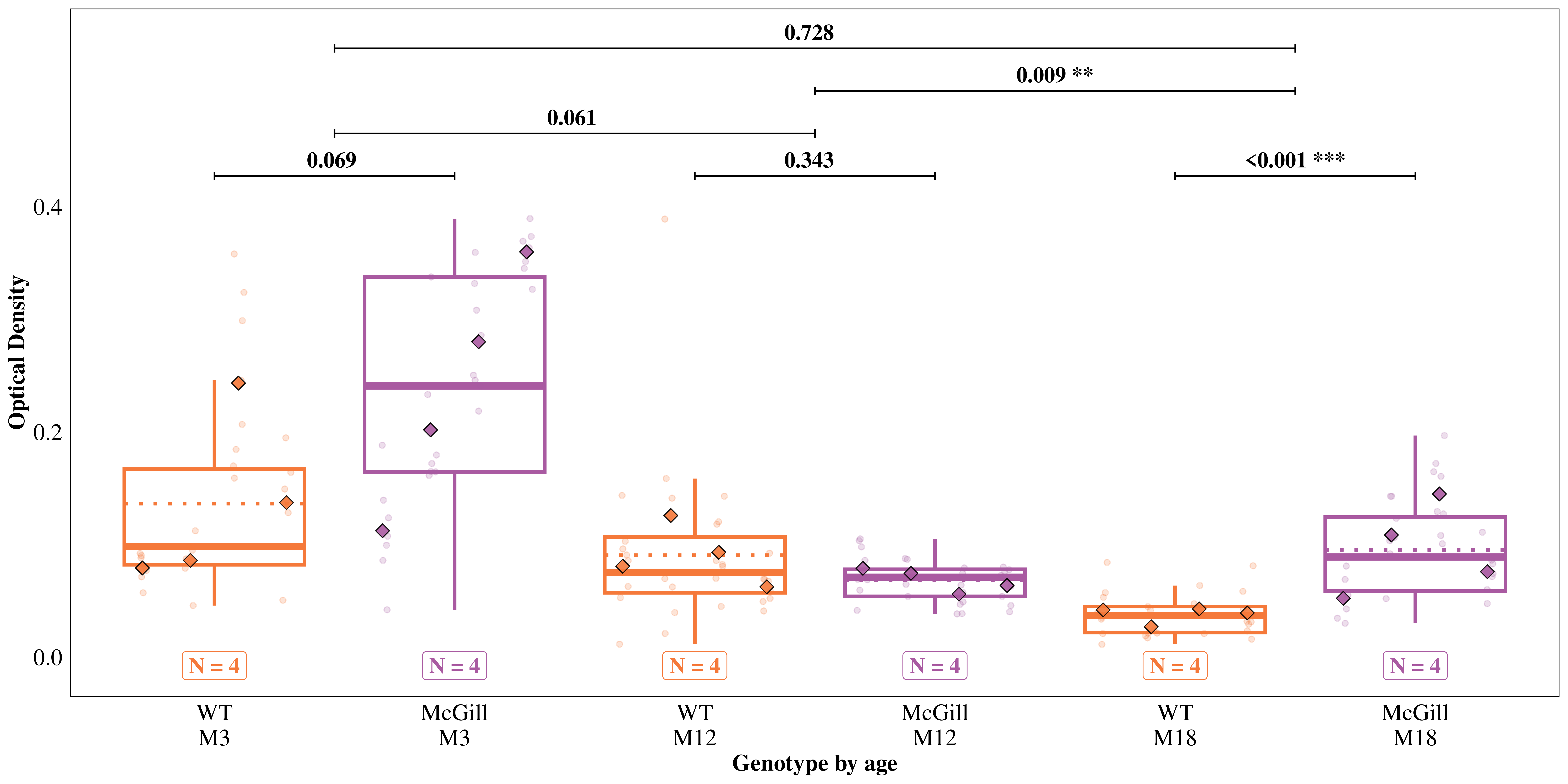
Tests are performed on the log scale

Annotated boxplots comparing BNIP3 expression in AD and control rats between age groups

We hypothesized that BNIP3 expression would be relatively low in other areas, but may be high in the projection areas of those neurons (CA3 & dentate gyrus). We used the ‘Molecular Layer’ model to test these hypotheses.

emmeans(mod_ml, specs = "genotype", type = "response") |> 
    contrast(method = "pairwise", adjust = "holm", infer = TRUE)

 contrast    ratio     SE  df asymp.LCL asymp.UCL null z.ratio p.value
 WT / McGill 0.715 0.0999 Inf     0.543      0.94    1  -2.403  0.0163

Results are averaged over the levels of: age 
Confidence level used: 0.95 
Intervals are back-transformed from the log scale 
Tests are performed on the log scale

Annotated boxplots comparing Optical Density in AD vs control rats for all age groups

emmeans(mod_ml, specs = ~ genotype | age, type = "response") |> 
    contrast(method = "pairwise", adjust = "none", infer = TRUE) |> 
    as.data.frame() |> 
    modify_at("p.value", \(x) p.adjust(x, method = "holm"))

age = M3:
 contrast     ratio     SE  df asymp.LCL asymp.UCL null z.ratio p.value
 WT / McGill 0.5610 0.1535 Inf    0.3281    0.9592    1  -2.112  0.0694

age = M12:
 contrast     ratio     SE  df asymp.LCL asymp.UCL null z.ratio p.value
 WT / McGill 1.2950 0.3529 Inf    0.7591    2.2091    1   0.949  0.3429

age = M18:
 contrast     ratio     SE  df asymp.LCL asymp.UCL null z.ratio p.value
 WT / McGill 0.5021 0.0823 Inf    0.3641    0.6924    1  -4.202  0.0001

Confidence level used: 0.95 
Intervals are back-transformed from the log scale 
Tests are performed on the log scale

emmeans(mod_ml, specs = ~ genotype | age, type = "response") |>
    contrast(interaction = "pairwise", by = NULL, adjust = "none", infer = TRUE) |> 
    as.data.frame() |> 
    modify_at("p.value", \(x) p.adjust(x, method = "holm"))

 genotype_pairwise age_pairwise  ratio     SE  df asymp.LCL asymp.UCL null z.ratio p.value
 WT / McGill        M3 / M12     0.4332 0.1673 Inf    0.2032     0.924    1  -2.166  0.0606
 WT / McGill        M3 / M18     1.1172 0.3564 Inf    0.5978     2.088    1   0.347  0.7283
 WT / McGill        M12 / M18    2.5788 0.8202 Inf    1.3826     4.810    1   2.979  0.0087

Confidence level used: 0.95 
Intervals are back-transformed from the log scale 
Tests are performed on the log scale

References

Brooks, M. E., Kristensen, K., van Benthem, K. J., Magnusson, A., Berg, C. W., Nielsen, A., Skaug, H. J., Maechler, M., & Bolker, B. M. (2017). glmmTMB balances speed and flexibility among packages for zero-inflated generalized linear mixed modeling. The R Journal, 9(2), 378–400. https://journal.r-project.org/archive/2017/RJ-2017-066/index.html

Hartig, F. (2022). DHARMa: Residual diagnostics for hierarchical (multi-level / mixed) regression models. https://CRAN.R-project.org/package=DHARMa

Lenth, R. V. (2022). Emmeans: Estimated marginal means, aka least-squares means. https://CRAN.R-project.org/package=emmeans

Lüdecke, D., Ben-Shachar, M. S., Patil, I., Waggoner, P., & Makowski, D. (2021). performance: An R package for assessment, comparison and testing of statistical models. Journal of Open Source Software, 6(60), 3139. https://doi.org/10.21105/joss.03139

Rodriguez-Duboc, A., Velicer, S. T., & Kobro-Flatmoen, A. (2025). Bnip3 expression in the brain of an Alzheimer’s disease rat model. Brain Mechanisms, 148–150, 202518. https://doi.org/10.1016/j.bramec.2025.202518